Zero Delay Feedback Filters in Reaktor

This tutorial relies heavily upon Zavalishin’s book. I have made an effort to condense it down to it’s most essential parts relating to zero delay feedback, and to make the material more accessible.

However, this is an advanced tutorial. It is assumed you have read and understood my previous tutorials on filter design (1, 2, 3), have a working understanding of the Reaktor Core environment, and have a decent recollection of high school algebra.

I’ll walk through the math step by step as much as I can, since in my own experience the biggest obstacle to understanding DSP papers is an expectation that the reader has a degree in engineering. It’s important to not gloss over the math in this tutorial if you wish to build your own zero delay filters.

One last thing before we start: I am a beginner in the world of zero delay feedback myself, so I apologize in advance for any inadvertant errors in this work.

WHY USE ZERO DELAY FILTERS?

One problem associated with the translation of analog filters into the digital domain is that the analog prototypes often contain a delayless loop. Zavalishin uses the following diagram of an analog one pole low pass as an example in his book:

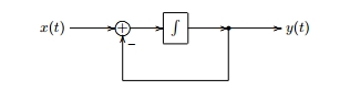
The ‘F’ block denotes an integrator, which is a common element in filter design.

Translating this diagram into the digital domain, we encounter a problem – in order to calculate the output, y(t), we must first calculate the input to the integrator. However, we can’t calculate the input to the integrator without first knowing the value of y(t), since the integrator takes an input value of x(t) – y(t).

A traditional way to solve this problem is to introduce a unit delay (known in core as the z^-1 module) into the feedback loop, leaving us with a digital version of the above diagram that looks like this:

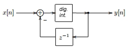
This way, we can simply subtract the previous output from the current input.

However, this creates another problem – the frequency response becomes warped, meaning the chosen cutoff point will not necessarily correspond to the actual cutoff point of the filter. The phase response will become warped as well.

Zero delay filters introduce a way to solve this problem without introducing the unit delay – leaving us with a better frequency response, and in my experience, improved behavior all around.

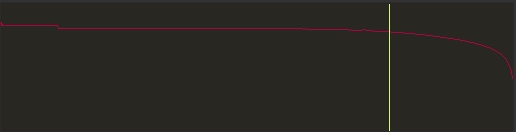
This graph illustrates this quite well:

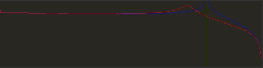
Here, the red line is the frequency response of a virtual MS-20 filter made using the bi-linear transform (I’ll make another tutorial soon on this topic) to convert from an analog prototype, by inserting a unit delay in the feedback path.

The blue line is the same filter, made using the zero delay technique, and the yellow line is the chosen frequency cutoff point. Both filters have their resonance set to max.

Notice how the zero delay version matches the cutoff point exactly, while the unit delay method is off by 2 kHz or more! Worse, the traditional version becomes unstable outside a certain frequency range, while the zero delay filter is stable across the spectrum. In the next tutorial, I will cover the creation of this filter.

INTEGRATOR TYPES

Before we can do much of anything with the filter diagram above, let’s talk about how to make a digital version of the integrator block. There are a few different ways to achieve this, but the type that seems to be favored by Zavalishin is the trapezoidal integrator (also called a bi-linear integrator), which has a Core structure that looks like this:

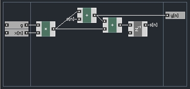
Where g is a variable dependent upon the cutoff point – we will go over g in full in a bit.

Here’s where things get interesting (and potentially confusing!). We define the input of the integrator as x[n], the output as y[n], and the output of the unit delay as s[n]. Therefore, we can say that

y[n] = gx[n] + s

Or, dropping the time notation for simplicity, simply

y = gx+s

ONE POLE LOW PASS

Now, let’s look again at the one pole filter. In fig 1, the input to the integrator is x-y. The output of the filter, y[n], is taken from the output of the integrator. Thus,

y[n] = g(x[n]-y[n]) + s

Okay, so we want to solve for the output of the filter, y[n]. The trouble with the above equation is that there is a y[n] on both sides of the equation so we can’t compute one side without knowing the value of the other. We can fix this, however. Ready for a bit of math?

Using the distributive property, and dropping the [n] notation for simplicity again, we can re-write the above equation as:

y = gx – gy + s

Then we arrange the equation such that all references to y are on the same side:

y + gy = gx + s

Next, we can factor out y from the left side ( IE – y+gy = y(1+g), like the distributive property in reverse, basically), leaving us with:

y(1+g) = gx+s

And finally, solving for y, we divide both sides by (1+g), leaving:

y = (gx+s)/(1+g)

This function gives us the output of the filter! In a strange quirk, we actually had to calculate the output of the filter before calculating the input to the integrator, which happens next. Here’s how it all looks (the TPT macro is the trapezoidal integrator):

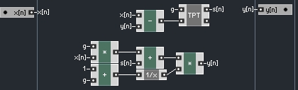
The trapezoidal integrator macro from above has been edited to output the value of s[n]. Notice that we no longer use the other output of the integrator to control anything, since we calculated that value (y) previously – the integrator’s purpose now is to update the value of s[n] for us in preparation for the next sample.

One other thing is required to make this structure work. In the function tab of properties, the TPT macro must have it’s ‘Solid’ parameter un-selected. If ‘Solid’ is set, it will stop the value of s from being sent at the correct time. For more on this subject, please check the Core manual section 5.4 – Feedback Around Macros, starting on page 113.

This structure gives us a simple low pass response:

CALCULATING G

Of course, none of this is worth much without a good method to control the value of g. Fortunately, this is easy. You can use two simple factory macros to do the job:

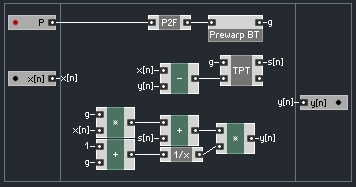
The P2F macro should be easy to find. The Prewarp BT macro can be found inside the 6dB LP/HP EQ macro. And of course, the ‘P’ input refers to the cutoff pitch.

Our filter so far looks like this:

CONCLUSION

There is still some further simplifications that can be made to improve this structure. Once complete, this one pole filter can be used as a building block to make more complex filters such as the MS-20 design mentioned above.

These subjects will be covered in the next tutorial, alongside a traditional version of the MS-20 filter for the sake of comparison.

As always, let me know if anything is unclear or needs to be covered in more detail.

For now, you can download a core macro of today’s work here.