Oversampling in Reaktor, Part I

WINDOWED SINC FILTER

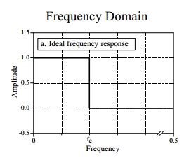
A windowed sinc filter is a digital approximation of an ‘ideal’ low pass filter. An ideal low pass will entirely cut out any spectral content above the cutoff frequency, with a frequency response that looks like this:

Click on image to see source document

By contrast, the filters encountered in synthesizers usually cut a signal by between 6 and 24 decibels per octave, a far more gradual cutoff.

Unfortunately, we cannot implement an ideal filter in a digital system like Reaktor – such a filter would require an infinite number of coefficients, among other problems. Instead we will work on getting something as close as possible to ideal.

We can start by defining the coefficients of a theoretical ideal filter, which can be calculated by the following function:

Click on image to see source document

Where fc is the cutoff frequency, and the i value represents the index of coefficients, and stretches from negative infinity to positive infinity.

This function is of the general form of the cardinal sine, or sinc, function, sin(x)/x, and while it consists mainly of values very close to zero, it does have non-zero values stretching out infinitely in both directions. The cardinal sine function:

Source: Wikipedia
Original Artist: Georg-Johann

In order to implement this filter in the digital domain, we must impose a window over the sinc function, hence the name windowed sinc filter.

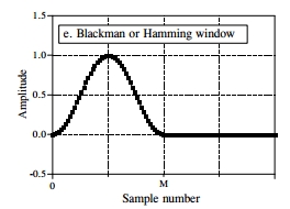
A window is a function that is equal to zero for most given inputs, except for a small range. The window we will use for today is the Blackman window, which has a graph that looks like this:

Click on image to see source document

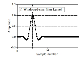
Since the function is equal to zero outside the range of 0 to 1, we can simply truncate most of the cardinal sine function by multiplying it against the window, leaving us with a graph that looks more like this:

Click on image to see source document

Now, we have a finite function defining our impulse response.

CREATING IT IN REAKTOR

To implement this filter, we need two pieces of information from the user – the cutoff frequency, and the number of taps, or coefficients, to use. The number of taps defines how many data points we will take from both the sinc function and blackman window function, and is directly related to how much CPU the filter will use.

Therefore, I used an iteration module that is triggered upon receiving a new cutoff value or number of coefficients:

The cutoff value (FC), number of taps -1 (M), and iteration index (I) are sent to the Windowed Sinc cell to do some work. The Order modules make sure that the current values for FC and M are received before the iteration begins.

Let’s move on the sinc function. First, we need to normalize the FC value, as is typical in filters. It should range from 0 to 0.5, hence we can simply divide the cutoff frequency by the sampling rate. Then our sinc macro looks like this.

There are a few things happening here. First, note that we end up subtracting M/2 from our incoming I value, which ranges from 0 to M. This value is then used as the I value in the sinc function listed above (Eq 1). We are sampling the sinc function then, from a range of -M/2 to M/2.

Second, if I – M/2 is equal to zero, the function will give an error (division by zero). Thus, we check to make sure the I and M/2 before moving forward.

The Blackman window must be computed also, and stretched to fit over the sinc function. The relevant area of the window ranges from 0 to 1, while the sinc function has M points. Therefore, we must collect M data points between 0 and 1 from the window function.
A Blackman window is defined as:

Where a0, a1, and a2 are known values.

In Reaktor this looks like:

The I/M module gives us the data point between 0 and 1 to sample from.

After using the incoming value I to sample a point from each function, we can multiply the values together and store the product as a coefficient to be used in the filter.

MODULAR CREATION

While a windowed sinc filter has some desirable properties, it’s lack of resonance and expensive coefficient calculation make it a bad fit for use as a standard audio shaping filter in a synth.

Instead, it has uses as an oversampling filter. In this instance, the coefficients will be constant and can be stored in a table. With this in mind, I created a simple macro to use for designing new filters in real time:

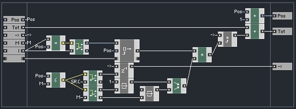
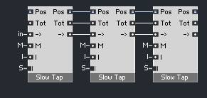
This macro has been designed to chain together multiple copies. Each copy represents one tap of the filter. The Pos, Tot, and -> values are passed from the output of one copy into the inputs of another like so:

The Pos value controls which coefficient is used for the tap, while the Tot value holds a running total of the sum of all previous taps. The -> holds the filter input, which gets multiplied by the coefficient and added to the running total. Finally, the input is delayed by a sample and sent to the output.

By linking several of these macros together in a chain, you are creating an FIR filter, where the Tot output of the final tap is the output of the filter. Note that this implementation is far from the most efficient realization of a windowed sinc filter. This is due to the fact that this macro contains a substantial amount of overhead that really is only necessary for testing purposes (giving us a variable number of taps to choose an optimal number for a final design).

A faster version might look something like this:

Although in this case we lose the ability to change the number of taps at will.

CONCLUSION

You can download a sample ensemble that demonstrates the use of the macros introduced in this tutorial here. The ensemble calculates and stores the coefficients of a filter specified by the user. The results are stored in an Event table where they can be saved as a text file and loaded in a Core table that can control the Data input of the Slow FIR macro, or better yet, a faster macro based upon the more efficient tap structure shown above.

In the next tutorial I will show how we can modify this structure to create a filter for use in oversampling.